Storing jaxvacua.vacuum objects

Storing `jaxvacua.vacuum` objects#

StringForge’s writers accept a jaxvacua.vacuum.Vacuum (or PFV / AFV) directly — no manual flattening to arrays. One call stores a list of vacua spanning any number of geometries, and read-back reconstructs the exact objects.

The authoritative record is the JSON-encoded Vacuum.to_dict() stashed in the free extra_data column (never pickle — the vault is public, so an unpickle-on-load would be a remote-code-execution vector). The typed columns (moduli, tau, flux, residual, W, N_flux, …) remain the queryable projection.

This notebook uses real vacua: dataset_B, 12196 solved \(h^{2,1}=2\) flux vacua for the degree-18 hypersurface in \(\mathbb{CP}^{1,1,1,6,9}\) (model_ID=1, \(Q_{D3}=276\)) — the literature-validation set used in the flux-bounding notebooks.

Setup#

import os, tempfile, gzip, pickle, json
from pathlib import Path
import numpy as np
import matplotlib.pyplot as plt

# Write to a throwaway vault so the tutorial never touches your real store.
os.environ['STRINGFORGE_VAULT'] = tempfile.mkdtemp()

import jaxvacua as jvc; jvc.set_precision('float64')
from jaxvacua.vacuum import Vacuum
from stringforge.lcs_database import LCSDatabase
print('jaxvacua', jvc.__version__)

jaxvacua 0.1.2

Load real vacua#

dataset_B ships as a gzip-pickled (12196, 18) array; each row is [x(6), flux(12)] — the real coordinate vector x (two complex moduli + the axio-dilaton) followed by the length-12 integer flux vector.

repo = Path(jvc.__file__).resolve().parents[1]
ds = repo/'documentation'/'source'/'notebooks'/'02_vacuum_finding'/'dataset_B.p'
with gzip.open(ds, 'rb') as f:
    A = pickle.load(f)
print(f'dataset_B: {A.shape[0]} real h12=2 vacua, layout [x(6), flux(12)]')

dataset_B: 12196 real h12=2 vacua, layout [x(6), flux(12)]

/var/folders/p7/f3t072gd3rbfgb00y3hj7dwc0000gn/T/ipykernel_87863/677447594.py:4: DeprecationWarning: numpy.core.numeric is deprecated and has been renamed to numpy._core.numeric. The numpy._core namespace contains private NumPy internals and its use is discouraged, as NumPy internals can change without warning in any release. In practice, most real-world usage of numpy.core is to access functionality in the public NumPy API. If that is the case, use the public NumPy API. If not, you are using NumPy internals. If you would still like to access an internal attribute, use numpy._core.numeric._frombuffer.
  A = pickle.load(f)

Build `Vacuum` objects#

We attach the model_ID=1 finder to recompute each vacuum’s diagnostics (\(W_0\), \(D_IW\), residual, \(g_s\)). The conifold diagnostics (zcf / alignment / residual_conifold) are None — legitimately not applicable to a pure-LCS vacuum — so every object is NaN-free.

finder = jvc.FluxVacuaFinder(h12=2, model_ID=1, maximum_degree=2)

def to_vacuum(row, tol=1e-4):
    x = np.asarray(row[:6], float); flux = np.asarray(row[6:18], float)
    z, _, tau, _ = finder._convert_real_to_complex(x)
    DW = np.asarray(finder.DW_x(x, flux)); res = float(np.max(np.abs(DW)))
    W0 = complex(finder.W(z, tau, flux, normalise=True))
    return Vacuum(x=x, flux=flux, W0=W0, DW=DW, residual=res,
                  residual_bulk=res, residual_conifold=None,
                  zcf=None, gs=float(1/tau.imag), alignment=None,
                  success=bool(res < tol), genealogy=['dataset_B'],
                  metadata={'model_name': 'CP11169_deg18'})

N = 250
vacua = [to_vacuum(A[i]) for i in range(N)]
print(f'built {len(vacua)} Vacuum objects | solved (res<1e-4): '
      f'{sum(v.is_solved() for v in vacua)}')

built 250 Vacuum objects | solved (res<1e-4): 206

Store them — one call#

db.write_vacua groups the vacua by geometry, opens one streaming writer per geometry, and returns a WriteReport. Passing models=finder lets it stamp the geometry-independent D3 tadpole N_flux = finder.tadpole(flux) on every row.

db = LCSDatabase(dataset='tdf', cache_dir=tempfile.mkdtemp(), offline=True)
report = db.write_vacua(vacua, models=finder)
print(report)
run_id = report.run_ids_by_geometry['CP11169_deg18']

WriteReport(n_written=206, n_duplicates=0, geometries=['CP11169_deg18'])

Read them back — exact#

db.read_vacua rebuilds the Vacuum objects from the stored record (finder-free). The queryable typed columns are still available through the unchanged load_vacua / query_vacua DataFrame path.

got = db.read_vacua(run_id)
# write_vacua stored the solved subset (only_solved=True); compare like-for-like
written = [v for v in vacua if v.is_solved()]
exact = all(a.equals(b) for a, b in zip(written, got))
print(f'read back {len(got)} Vacuum objects (the solved subset) | all exact: {exact}')

dfq = db.load_vacua(run_id)
cols = ['flux','moduli_re','moduli_im','tau_re','tau_im','N_flux','W_re','residual']
print('queryable columns:', [c for c in cols if c in dfq.columns])
dfq[['tau_im','N_flux','W_re','residual']].head()

read back 206 Vacuum objects (the solved subset) | all exact: True
queryable columns: ['flux', 'moduli_re', 'moduli_im', 'tau_re', 'tau_im', 'N_flux', 'W_re', 'residual']

	tau_im	N_flux	W_re	residual
0	1.005013	9	-42.117417	0.000001
1	1.005013	9	42.117417	0.000001
2	1.246215	10	5.112692	0.000028
3	1.246215	10	-5.112692	0.000028
4	1.270350	10	20.650255	0.000003

The stored ensemble#

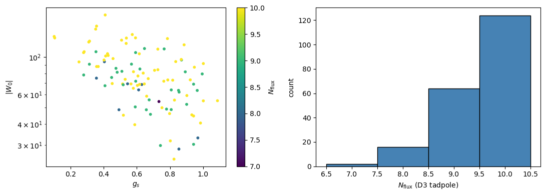
Because the typed projection is queryable, the stored run is immediately plottable — here the \((g_s, |W_0|)\) distribution coloured by D3 tadpole, and the tadpole histogram.

gs    = np.array([v.gs for v in got])
absW0 = np.array([abs(v.W0) for v in got])
Nflux = np.asarray(dfq['N_flux'], dtype=float)

fig, ax = plt.subplots(1, 2, figsize=(11, 4))
sc = ax[0].scatter(gs, absW0, c=Nflux, cmap='viridis', s=16, edgecolor='none')
ax[0].set_xlabel(r'$g_s$'); ax[0].set_ylabel(r'$|W_0|$'); ax[0].set_yscale('log')
plt.colorbar(sc, ax=ax[0], label=r'$N_{\rm flux}$')

lo, hi = int(np.nanmin(Nflux)), int(np.nanmax(Nflux))
ax[1].hist(Nflux, bins=range(lo, hi + 2), color='steelblue', edgecolor='k', align='left')
ax[1].set_xlabel(r'$N_{\rm flux}$ (D3 tadpole)'); ax[1].set_ylabel('count')
fig.tight_layout(); plt.show()

../_images/0f07930db1b4daa888f6a24b15cb22ec17ef5b1f51dba2cf51b7e42c9bf58d55.png

The record is JSON, not pickle#

The exact object travels in extra_data as JSON — inspectable, portable, and safe to load from an untrusted source.

blob = json.loads(dfq['extra_data'].iloc[0])
print('extra_data keys :', list(blob.keys()))
print('record _kind    :', blob['vacuum']['_kind'])
print('round-trips exact:', got[0].equals(vacua[0]))

extra_data keys : ['vacuum', 'kind', 'model_name']
record _kind    : Vacuum
round-trips exact: True

Production tier (Vulcan)#

The same adapter backs the high-volume vulcan writer, which stages parquet shards for HuggingFace publishing:

from stringforge.vulcan import Vulcan
vulc = Vulcan(repo='your-org/your-dataset')
shard = vulc.write_vacua(vacua, finder=finder)   # one shard per geometry
back  = vulc.read_vacua(shard)                    # exact reconstruction

Summary#

db.write_vacua(vacua, models=finder) / db.read_vacua(run_id) store and reconstruct Vacuum objects exactly, in one call.
Advanced streaming: with db.vacua_writer(model=finder) as w: w.append(vac).
The record is JSON in extra_data (no pickle); the typed columns stay queryable; the production vulcan tier mirrors the same API.